
- CHAPTER 0: Neural Networks and Deep Learning
- CHAPTER 1: Using neural nets to recognize handwritten digits
CHAPTER 0: Neural Networks and Deep Learning
Neural Networks and Deep Learning is a free online book written by Michael Nielsen. I asked Micheal for permission to rewrite his book in R (the original book is in python found here). I had to learn python to be able to completely benefit from Michael’s incredible book. So I took it upon myself to rewrite the book in R so you will not have to learn python if you are already an R programmer. From time to time I will add something called the StatsNotes which relates the terminology used in this book to traditional statistical methods.
The book will teach you about:
- Neural networks, a beautiful biologically-inspired programming paradigm which enables a computer to learn from observational data
- Deep learning, a powerful set of techniques for learning in neural networks
Neural networks and deep learning currently provide the best solutions to many problems in image recognition, speech recognition, and natural language processing. This book will teach you many of the core concepts behind neural networks and deep learning.
For more details about the approach taken in the book, see here. Or you can jump directly to Chapter 1 and get started.
What this book is about
Neural networks are one of the most beautiful programming paradigms ever invented. In the conventional approach to programming, we tell the computer what to do, breaking big problems up into many small, precisely defined tasks that the computer can easily perform. By contrast, in a neural network we don’t tell the computer how to solve our problem. Instead, it learns from observational data, figuring out its own solution to the problem at hand.
Automatically learning from data sounds promising. However, until 2006 we didn’t know how to train neural networks to surpass more traditional approaches, except for a few specialized problems. What changed in 2006 was the discovery of techniques for learning in so-called deep neural networks. These techniques are now known as deep learning. They’ve been developed further, and today deep neural networks and deep learning achieve outstanding performance on many important problems in computer vision, speech recognition, and natural language processing. They’re being deployed on a large scale by companies such as Google, Microsoft, and Facebook.
The purpose of this book is to help you master the core concepts of neural networks, including modern techniques for deep learning. After working through the book you will have written code that uses neural networks and deep learning to solve complex pattern recognition problems. And you will have a foundation to use neural networks and deep learning to attack problems of your own devising.
A principle-oriented approach
One conviction underlying the book is that it’s better to obtain a solid understanding of the core principles of neural networks and deep learning, rather than a hazy understanding of a long laundry list of ideas. If you’ve understood the core ideas well, you can rapidly understand other new material. In programming language terms, think of it as mastering the core syntax, libraries and data structures of a new language. You may still only “know” a tiny fraction of the total language - many languages have enormous standard libraries - but new libraries and data structures can be understood quickly and easily.
This means the book is emphatically not a tutorial in how to use some particular neural network library. If you mostly want to learn your way around a library, don’t read this book! Find the library you wish to learn, and work through the tutorials and documentation. But be warned. While this has an immediate problem-solving payoff, if you want to understand what’s really going on in neural networks, if you want insights that will still be relevant years from now, then it’s not enough just to learn some hot library. You need to understand the durable, lasting insights underlying how neural networks work. Technologies come and technologies go, but insight is forever.
A hands-on approach
We’ll learn the core principles behind neural networks and deep learning by attacking a concrete problem: the problem of teaching a computer to recognize handwritten digits. This problem is extremely difficult to solve using the conventional approach to programming. And yet, as we’ll see, it can be solved pretty well using a simple neural network, with just a few tens of lines of code, and no special libraries. What’s more, we’ll improve the program through many iterations, gradually incorporating more and more of the core ideas about neural networks and deep learning.
This hands-on approach means that you’ll need some programming experience to read the book. But you don’t need to be a professional programmer. The original version of this book was written in Python (version 2.7), which, even if you don’t program in Python, should be easy to understand with just a little effort. However, this version of the book is written in R to make it easier for R programmers. Through the course of the book we will develop a little neural network library, which you can use to experiment and to build understanding. All the code is available for download here. Once you’ve finished the book, or as you read it, you can easily pick up one of the more feature-complete neural network libraries intended for use in production.
On a related note, the mathematical requirements to read the book are modest. There is some mathematics in most chapters, but it’s usually just elementary algebra and plots of functions, which I expect most readers will be okay with. I occasionally use more advanced mathematics, but have structured the material so you can follow even if some mathematical details elude you. The one chapter which uses heavier mathematics extensively is Chapter 2, which requires a little multivariable calculus and linear algebra. If those aren’t familiar, I begin Chapter 2 with a discussion of how to navigate the mathematics. If you’re finding it really heavy going, you can simply skip to the summary of the chapter’s main results. In any case, there’s no need to worry about this at the outset.
It’s rare for a book to aim to be both principle-oriented and hands-on. But I believe you’ll learn best if we build out the fundamental ideas of neural networks. We’ll develop living code, not just abstract theory, code which you can explore and extend. This way you’ll understand the fundamentals, both in theory and practice, and be well set to add further to your knowledge.
On the exercises and problems
It’s not uncommon for technical books to include an admonition from the author that readers must do the exercises and problems. I always feel a little peculiar when I read such warnings. Will something bad happen to me if I don’t do the exercises and problems? Of course not. I’ll gain some time, but at the expense of depth of understanding. Sometimes that’s worth it. Sometimes it’s not.
So what’s worth doing in this book? My advice is that you really should attempt most of the exercises, and you should aim not to do most of the problems.
You should do most of the exercises because they’re basic checks that you’ve understood the material. If you can’t solve an exercise relatively easily, you’ve probably missed something fundamental. Of course, if you do get stuck on an occasional exercise, just move on - chances are it’s just a small misunderstanding on your part, or maybe I’ve worded something poorly. But if most exercises are a struggle, then you probably need to reread some earlier material.
The problems are another matter. They’re more difficult than the exercises, and you’ll likely struggle to solve some problems. That’s annoying, but, of course, patience in the face of such frustration is the only way to truly understand and internalize a subject.
With that said, I don’t recommend working through all the problems. What’s even better is to find your own project. Maybe you want to use neural nets to classify your music collection. Or to predict stock prices. Or whatever. But find a project you care about. Then you can ignore the problems in the book, or use them simply as inspiration for work on your own project. Struggling with a project you care about will teach you far more than working through any number of set problems. Emotional commitment is a key to achieving mastery.
Of course, you may not have such a project in mind, at least up front. That’s fine. Work through those problems you feel motivated to work on. And use the material in the book to help you search for ideas for creative personal projects.
CHAPTER 1: Using neural nets to recognize handwritten digits
The human visual system is one of the wonders of the world. Consider the following sequence of handwritten digits:
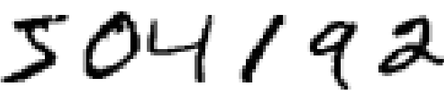
Most people effortlessly recognize those digits as 504192. That ease is deceptive. In each hemisphere of our brain, humans have a primary visual cortex, also known as V1, containing 140 million neurons, with tens of billions of connections between them. And yet human vision involves not just V1, but an entire series of visual cortices - V2, V3, V4, and V5 - doing progressively more complex image processing. We carry in our heads a supercomputer, tuned by evolution over hundreds of millions of years, and superbly adapted to understand the visual world. Recognizing handwritten digits isn’t easy. Rather, we humans are stupendously, astoundingly good at making sense of what our eyes show us. But nearly all that work is done unconsciously. And so we don’t usually appreciate how tough a problem our visual systems solve.
The difficulty of visual pattern recognition becomes apparent if you attempt to write a computer program to recognize digits like those above. What seems easy when we do it ourselves suddenly becomes extremely difficult. Simple intuitions about how we recognize shapes - “a 9 has a loop at the top, and a vertical stroke in the bottom right” - turn out to be not so simple to express algorithmically. When you try to make such rules precise, you quickly get lost in a morass of exceptions and caveats and special cases. It seems hopeless.
Neural networks approach the problem in a different way. The idea is to take a large number of handwritten digits, known as training examples,
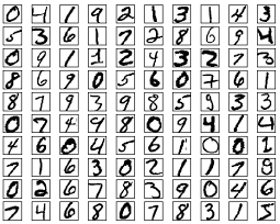
and then develop a system which can learn from those training examples. In other words, the neural network uses the examples to automatically infer rules for recognizing handwritten digits. Furthermore, by increasing the number of training examples, the network can learn more about handwriting, and so improve its accuracy. So while I’ve shown just 100 training digits above, perhaps we could build a better handwriting recognizer by using thousands or even millions or billions of training examples.
In this chapter we’ll write a computer program implementing a neural network that learns to recognize handwritten digits. The program is just 74 lines long, and uses no special neural network libraries. But this short program can recognize digits with an accuracy over 96 percent, without human intervention. Furthermore, in later chapters we’ll develop ideas which can improve accuracy to over 99 percent. In fact, the best commercial neural networks are now so good that they are used by banks to process cheques, and by post offices to recognize addresses.
We’re focusing on handwriting recognition because it’s an excellent prototype problem for learning about neural networks in general. As a prototype it hits a sweet spot: it’s challenging - it’s no small feat to recognize handwritten digits - but it’s not so difficult as to require an extremely complicated solution, or tremendous computational power. Furthermore, it’s a great way to develop more advanced techniques, such as deep learning. And so throughout the book we’ll return repeatedly to the problem of handwriting recognition. Later in the book, we’ll discuss how these ideas may be applied to other problems in computer vision, and also in speech, natural language processing, and other domains.
Of course, if the point of the chapter was only to write a computer program to recognize handwritten digits, then the chapter would be much shorter! But along the way we’ll develop many key ideas about neural networks, including two important types of artificial neuron (the perceptron and the sigmoid neuron), and the standard learning algorithm for neural networks, known as stochastic gradient descent. Throughout, I focus on explaining why things are done the way they are, and on building your neural networks intuition. That requires a lengthier discussion than if I just presented the basic mechanics of what’s going on, but it’s worth it for the deeper understanding you’ll attain. Amongst the payoffs, by the end of the chapter we’ll be in position to understand what deep learning is, and why it matters.
Perceptrons
What is a neural network? To get started, I’ll explain a type of artificial neuron called a perceptron. Perceptrons were developed in the 1950s and 1960s by the scientist Frank Rosenblatt, inspired by earlier work by Warren McCulloch and Walter Pitts. Today, it’s more common to use other models of artificial neurons - in this book, and in much modern work on neural networks, the main neuron model used is one called the sigmoid neuron. We’ll get to sigmoid neurons shortly. But to understand why sigmoid neurons are defined the way they are, it’s worth taking the time to first understand perceptrons.
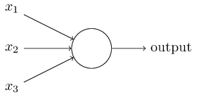
So how do perceptrons work? A perceptron takes several binary inputs, \(x_1,x_2,\ldots\), and produces a single binary output:

In the example shown the perceptron has three inputs, \(x_1,x_2,x_3\) . In general it could have more or fewer inputs. Rosenblatt proposed a simple rule to compute the output. He introduced weights, \(w_1,w_2,\ldots\), real numbers expressing the importance of the respective inputs to the output. The neuron’s output, 0 or 1, is determined by whether the weighted sum \(\sum_j w_j x_j\) is less than or greater than some threshold value. Just like the weights, the threshold is a real number which is a parameter of the neuron. To put it in more precise algebraic terms:
\[\text{output}= \begin{cases} 0 ~~~\text{if} ~~\sum_j w_j x_j \leq \text{threshold} ~~~~ (1)\\ 1 ~~~\text{if} ~~\sum_j w_j x_j > \text{threshold}\\ \end{cases}\]That’s all there is to how a perceptron works!
That’s the basic mathematical model. A way you can think about the perceptron is that it’s a device that makes decisions by weighing up evidence. Let me give an example. It’s not a very realistic example, but it’s easy to understand, and we’ll soon get to more realistic examples. Suppose the weekend is coming up, and you’ve heard that there’s going to be a cheese festival in your city. You like cheese, and are trying to decide whether or not to go to the festival. You might make your decision by weighing up three factors:
- Is the weather good?
- Does your boyfriend or girlfriend want to accompany you?
- Is the festival near public transit? (You don’t own a car).
We can represent these three factors by corresponding binary variables \(x_1,x_2\), and \(x_3\). For instance, we’d have \(x_1=1\) if the weather is good, and \(x_1=0\) if the weather is bad. Similarly, \(x_2=1\) if your boyfriend or girlfriend wants to go, and \(x_2=0\) if not. And similarly again for \(x_3\) and public transit.
Now, suppose you absolutely adore cheese, so much so that you’re happy to go to the festival even if your boyfriend or girlfriend is uninterested and the festival is hard to get to. But perhaps you really loathe bad weather, and there’s no way you’d go to the festival if the weather is bad. You can use perceptrons to model this kind of decision-making. One way to do this is to choose a weight \(w_1=6\) for the weather, and \(w_2=2\) and \(w_3=2\) for the other conditions. The larger value of \(w_1\) indicates that the weather matters a lot to you, much more than whether your boyfriend or girlfriend joins you, or the nearness of public transit. Finally, suppose you choose a threshold of 5 for the perceptron. With these choices, the perceptron implements the desired decision-making model, outputting 1 whenever the weather is good, and 0 whenever the weather is bad. It makes no difference to the output whether your boyfriend or girlfriend wants to go, or whether public transit is nearby.
By varying the weights and the threshold, we can get different models of decision-making. For example, suppose we instead chose a threshold of 3. Then the perceptron would decide that you should go to the festival whenever the weather was good or when both the festival was near public transit and your boyfriend or girlfriend was willing to join you. In other words, it’d be a different model of decision-making. Dropping the threshold means you’re more willing to go to the festival.
Obviously, the perceptron isn’t a complete model of human decision-making! But what the example illustrates is how a perceptron can weigh up different kinds of evidence in order to make decisions. And it should seem plausible that a complex network of perceptrons could make quite subtle decisions:
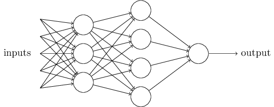
In this network, the first column of perceptrons - what we’ll call the first layer of perceptrons - is making three very simple decisions, by weighing the input evidence. What about the perceptrons in the second layer? Each of those perceptrons is making a decision by weighing up the results from the first layer of decision-making. In this way a perceptron in the second layer can make a decision at a more complex and more abstract level than perceptrons in the first layer. And even more complex decisions can be made by the perceptron in the third layer. In this way, a many-layer network of perceptrons can engage in sophisticated decision making.
Incidentally, when I defined perceptrons I said that a perceptron has just a single output. In the network above the perceptrons look like they have multiple outputs. In fact, they’re still single output. The multiple output arrows are merely a useful way of indicating that the output from a perceptron is being used as the input to several other perceptrons. It’s less unwieldy than drawing a single output line which then splits.
Let’s simplify the way we describe perceptrons. The condition \(\sum_jw_jx_j>\) threshold is cumbersome, and we can make two notational changes to simplify it. The first change is to write \(\sum_jw_jx_j\) as a dot product, \(w⋅x=\sum_j w_j x_j\), where \(w\) and \(x\) are vectors whose components are the weights and inputs, respectively. The second change is to move the threshold to the other side of the inequality, and to replace it by what’s known as the perceptron’s bias, \(b=−\) threshold. Using the bias instead of the threshold, the perceptron rule can be rewritten:
\[\text{output}=\begin{cases} 0 & \text{if } w.x+b \leq 0~~~ (2)\\ 1 & \text{if } w.x+b > 0 \end{cases}\]You can think of the bias as a measure of how easy it is to get the perceptron to output a 1. Or to put it in more biological terms, the bias is a measure of how easy it is to get the perceptron to fire. For a perceptron with a really big bias, it’s extremely easy for the perceptron to output a 1. But if the bias is very negative, then it’s difficult for the perceptron to output a 1. Obviously, introducing the bias is only a small change in how we describe perceptrons, but we’ll see later that it leads to further notational simplifications. Because of this, in the remainder of the book we won’t use the threshold, we’ll always use the bias.
I’ve described perceptrons as a method for weighing evidence to make decisions. Another way perceptrons can be used is to compute the elementary logical functions we usually think of as underlying computation, functions such as AND, OR, and NAND. For example, suppose we have a perceptron with two inputs, each with weight −2, and an overall bias of 3. Here’s our perceptron:
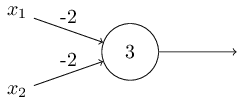
Then we see that input 00 produces output 1, since \((−2)\times0+(−2)\times0+3=3\) is positive. Here, I’ve introduced the ∗ symbol to make the multiplications explicit. Similar calculations show that the inputs 01 and 10 produce output 1. But the input 11 produces output 0, since \((−2)\times 1+(−2)\times 1+3=−1\) is negative. And so our perceptron implements a NAND gate!
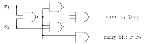
The NAND example shows that we can use perceptrons to compute simple logical functions. In fact, we can use networks of perceptrons to compute any logical function at all. The reason is that the NAND gate is universal for computation, that is, we can build any computation up out of NAND gates. For example, we can use NAND gates to build a circuit which adds two bits, \(x_1\) and \(x_2\). This requires computing the bitwise sum, \(x_1\oplus x_2\), as well as a carry bit which is set to 1 when both \(x_1\) and \(x_2\) are 1, i.e., the carry bit is just the bitwise product \(x_1x_2\):
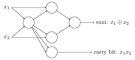
 To get an equivalent network of perceptrons we replace all the NAND gates by perceptrons with two inputs, each with weight −2, and an overall bias of 3. Here’s the resulting network. Note that I’ve moved the perceptron corresponding to the bottom right NAND gate a little, just to make it easier to draw the arrows on the diagram:
The computational universality of perceptrons is simultaneously reassuring and disappointing. It’s reassuring because it tells us that networks of perceptrons can be as powerful as any other computing device. But it’s also disappointing, because it makes it seem as though perceptrons are merely a new type of NAND gate. That’s hardly big news!
However, the situation is better than this view suggests. It turns out that we can devise learning algorithms which can automatically tune the weights and biases of a network of artificial neurons. This tuning happens in response to external stimuli, without direct intervention by a programmer. These learning algorithms enable us to use artificial neurons in a way which is radically different to conventional logic gates. Instead of explicitly laying out a circuit of NAND and other gates, our neural networks can simply learn to solve problems, sometimes problems where it would be extremely difficult to directly design a conventional circuit.
StatsNotes
In traditional statistical terms \(w\) are the variable coefficients as usually denoted with \(\beta\) while the bias \(b\) is often call the intercept.
Sigmoid neurons
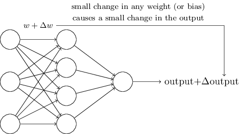
Learning algorithms sound terrific. But how can we devise such algorithms for a neural network? Suppose we have a network of perceptrons that we’d like to use to learn to solve some problem. For example, the inputs to the network might be the raw pixel data from a scanned, handwritten image of a digit. And we’d like the network to learn weights and biases so that the output from the network correctly classifies the digit. To see how learning might work, suppose we make a small change in some weight (or bias) in the network. What we’d like is for this small change in weight to cause only a small corresponding change in the output from the network. As we’ll see in a moment, this property will make learning possible. Schematically, here’s what we want (obviously this network is too simple to do handwriting recognition!):
If it were true that a small change in a weight (or bias) causes only a small change in output, then we could use this fact to modify the weights and biases to get our network to behave more in the manner we want. For example, suppose the network was mistakenly classifying an image as an “8” when it should be a “9”. We could figure out how to make a small change in the weights and biases so the network gets a little closer to classifying the image as a “9”. And then we’d repeat this, changing the weights and biases over and over to produce better and better output. The network would be learning.
The problem is that this isn’t what happens when our network contains perceptrons. In fact, a small change in the weights or bias of any single perceptron in the network can sometimes cause the output of that perceptron to completely flip, say from 0 to 1. That flip may then cause the behaviour of the rest of the network to completely change in some very complicated way. So while your “9” might now be classified correctly, the behaviour of the network on all the other images is likely to have completely changed in some hard-to-control way. That makes it difficult to see how to gradually modify the weights and biases so that the network gets closer to the desired behaviour. Perhaps there’s some clever way of getting around this problem. But it’s not immediately obvious how we can get a network of perceptrons to learn.
We can overcome this problem by introducing a new type of artificial neuron called a sigmoid neuron. Sigmoid neurons are similar to perceptrons, but modified so that small changes in their weights and bias cause only a small change in their output. That’s the crucial fact which will allow a network of sigmoid neurons to learn.
Okay, let me describe the sigmoid neuron. We’ll depict sigmoid neurons in the same way we depicted perceptrons:
Just like a perceptron, the sigmoid neuron has inputs, \(x_1,x_2,\ldots\). But instead of being just 0 or 1, these inputs can also take on any values between 0 and 1. So, for instance, 0.638 is a valid input for a sigmoid neuron. Also just like a perceptron, the sigmoid neuron has weights for each input, \(w1,w2,\ldots\), and an overall bias, \(b\). But the output is not 0 or 1. Instead, it’s \(\sigma (w⋅x+b)\), where \(\sigma\) is called the sigmoid function. and is defined by:
\[\sigma(z)=\frac{1}{1+e^{-z}}~~~ (3)\]StatsNotes
Can statisticians already guess what we are getting at here? Of course a sigmoid neuron is a logistic regression model. Now if we will replace \(\sigma\) with the cummulative normal distribution function \(\Phi\), this will be a probit model. In general these functions are called activation functions. In statistics, in the context of generalised linear models, activation functions are simply link functions or inverse link functions. The question is, if neural networks are simply generalised linear models, what is all this hype about?
To put it all a little more explicitly, the output of a sigmoid neuron with inputs \(x_1,x_2,\ldots\), weights \(w_1,w_2,\ldots\), and bias \(b\) is
\[\frac{1}{1+\exp(-\sum_j w_j x_j)} ~~~(4)\]At first sight, sigmoid neurons appear very different to perceptrons. The algebraic form of the sigmoid function may seem opaque and forbidding if you’re not already familiar with it. In fact, there are many similarities between perceptrons and sigmoid neurons, and the algebraic form of the sigmoid function turns out to be more of a technical detail than a true barrier to understanding.
To understand the similarity to the perceptron model, suppose \(z=w⋅x+b\) is a large positive number. Then \(e^{−z}\approx\) and so \(\sigma(z)\approx 1\). In other words, when \(z=w⋅x+b\) is large and positive, the output from the sigmoid neuron is approximately 1, just as it would have been for a perceptron. Suppose on the other hand that \(z=w⋅x+b\) is very negative. Then \(e^{-z}\rightarrow \infty\), and \(\sigma (z)\approx 0\). So when \(z=w⋅x+b\) is very negative, the behaviour of a sigmoid neuron also closely approximates a perceptron. It’s only when \(w⋅x+b\) is of modest size that there’s much deviation from the perceptron model.
What about the algebraic form of \(\sigma\)? How can we understand that? In fact, the exact form of \(\sigma\) isn’t so important - what really matters is the shape of the function when plotted. Here’s the shape:
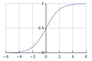
This shape is a smoothed out version of a step function:
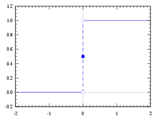
If \(\sigma\) had in fact been a step function, then the sigmoid neuron would be a perceptron, since the output would be 1 or 0 depending on whether \(w⋅x+b\) was positive or negative.
Actually, when \(w⋅x+b=0\) the perceptron outputs 0, while the step function outputs 1. So, strictly speaking, we’d need to modify the step function at that one point. But you get the idea.
By using the actual \(\sigma\) function we get, as already implied above, a smoothed out perceptron. Indeed, it’s the smoothness of the \(\sigma\) function that is the crucial fact, not its detailed form. The smoothness of \(\sigma\) means that small changes \(\Delta w_j\) in the weights and \(\Delta b\) in the bias will produce a small change \(\Delta\)output in the output from the neuron. In fact, calculus tells us that \(\Delta\)output is well approximated by
\[\Delta \text{output}\approx \sum_j \frac{\partial \text{output}}{\partial w_j}\Delta w_j + \frac{\partial \text{output}}{\partial b}\Delta b ~~~ (5)\]where the sum is over all the weights, \(w_j\), and \(\partial \text{output}/\partial w_j\) and \(\partial \text{output}/\partial b\) denote partial derivatives of the output with respect to \(w_j\) and \(b\), respectively. Don’t panic if you’re not comfortable with partial derivatives! While the expression above looks complicated, with all the partial derivatives, it’s actually saying something very simple (and which is very good news): \(\Delta\)output is a linear function of the changes \(\Delta w_j\) and \(\Delta b\) in the weights and bias. This linearity makes it easy to choose small changes in the weights and biases to achieve any desired small change in the output. So while sigmoid neurons have much of the same qualitative behaviour as perceptrons, they make it much easier to figure out how changing the weights and biases will change the output.
If it’s the shape of \(\sigma\) which really matters, and not its exact form, then why use the particular form used for \(\sigma\) in Equation (3)? In fact, later in the book we will occasionally consider neurons where the output is \(f(w⋅x+b)\) for some other activation function \(f(⋅)\). The main thing that changes when we use a different activation function is that the particular values for the partial derivatives in Equation (5) change. It turns out that when we compute those partial derivatives later, using \(\sigma\) will simplify the algebra, simply because exponentials have lovely properties when differentiated. In any case, \(\sigma\) is commonly-used in work on neural nets, and is the activation function we’ll use most often in this book.
How should we interpret the output from a sigmoid neuron? Obviously, one big difference between perceptrons and sigmoid neurons is that sigmoid neurons don’t just output 0 or 1. They can have as output any real number between 0 and 1, so values such as 0.173 and 0.689 are legitimate outputs. This can be useful, for example, if we want to use the output value to represent the average intensity of the pixels in an image input to a neural network. But sometimes it can be a nuisance. Suppose we want the output from the network to indicate either “the input image is a 9” or “the input image is not a 9”. Obviously, it’d be easiest to do this if the output was a 0 or a 1, as in a perceptron. But in practice we can set up a convention to deal with this, for example, by deciding to interpret any output of at least 0.5 as indicating a “9”, and any output less than 0.5 as indicating “not a 9”. I’ll always explicitly state when we’re using such a convention, so it shouldn’t cause any confusion.
Exercises
Sigmoid neurons simulating perceptrons, part I
Suppose we take all the weights and biases in a network of perceptrons, and multiply them by a positive constant, \(c>0\). Show that the behaviour of the network doesn’t change.
Sigmoid neurons simulating perceptrons, part II
Suppose we have the same setup as the last problem - a network of perceptrons. Suppose also that the overall input to the network of perceptrons has been chosen. We won’t need the actual input value, we just need the input to have been fixed. Suppose the weights and biases are such that \(w⋅x+b\neq 0\) for the input \(x\) to any particular perceptron in the network. Now replace all the perceptrons in the network by sigmoid neurons, and multiply the weights and biases by a positive constant \(c>0\). Show that in the limit as \(c\rightarrow \infty\) the behaviour of this network of sigmoid neurons is exactly the same as the network of perceptrons. How can this fail when \(w⋅x+b=0\) for one of the perceptrons?