
Anomaly detection with autoencoders
In this blog post we will use autoencoders to detect anomalies in ECG5000 dataset. In writing this blog post I have assumed that the reader has some basic understanding of neural networks and autoencoders as a specific type of neural network. Jeremy Jordan has a nice 10mins-read blog post on autoencoders, you can find it here. The ECG5000 dataset which we will use contains 50,000 Electrocardiograms (ECG). Each cardiogram has 140 data points. Luckily for us, the data has been labeled into a normal and abnormal rhythm by medical experts. Our goal is to use autoencoders to see if they can mimic the knowledge of a medical doctor and identify abnormal Electrocardiograms.

Our approach will be to (1) train the autoencoder on the normal data and (2) use our trained model to reconstruct the entire dataset. We hypothesize that abnormal Electrocardiograms will have a higher reconstruction error. Recall that an autoencoder takes the input data and projects it onto a lower-dimensional space that captures only the signals in the data. The data can then be reconstructed from the lower-dimensional space. Note here that if a data point is noisy its reconstruction error (the distance between the actual point and the reconstructed one) will be large. It is this simple principle that we use to identity anomalies.
Lets load the ECG data
# libraries
import matplotlib.pyplot as plt
import numpy as np
import pandas as pd
import tensorflow as tf


from sklearn.model_selection import train_test_split
from sklearn.metrics import accuracy_score, precision_score, recall_score
from tensorflow.keras import layers, losses
from tensorflow.keras.datasets import fashion_mnist
from tensorflow.keras.models import Model
import plotly.express as px
import plotly.graph_objects as go
import plotly.offline as py_offline
# Download the dataset
url = 'http://storage.googleapis.com/download.tensorflow.org/data/ecg.csv'

dataframe = pd.read_csv(url,header=None)
raw_data = dataframe.values
# first five rows and columns
print(dataframe.iloc[:,0:5].head().to_markdown())
|    |         0 |         1 |        2 |        3 |        4 |
|---:|----------:|----------:|---------:|---------:|---------:|
|  0 | -0.112522 | -2.8272   | -3.7739  | -4.34975 | -4.37604 |
|  1 | -1.10088  | -3.99684  | -4.28584 | -4.50658 | -4.02238 |
|  2 | -0.567088 | -2.59345  | -3.87423 | -4.58409 | -4.18745 |
|  3 |  0.490473 | -1.91441  | -3.61636 | -4.31882 | -4.26802 |
|  4 |  0.800232 | -0.874252 | -2.38476 | -3.97329 | -4.33822 |
The last column contains the labels. The other data points are the electrocardiogram data. We will also create a train and test a dataset, as well as their labels, this is what data scientists do to overcome a serious problem in data science namely over-fitting.
# The last element contains the labels
labels = raw_data[:, -1]

# The other data points are the electrocadriogram data
data = raw_data[:, 0:-1]

train_data, test_data, train_labels, test_labels = train_test_split(
    data, labels, test_size=0.2, random_state=21
)
We will also normalize the data to lie between [0,1]. Note here that we do normalization because to speed up the learning and convergence of the optimizer.
min_val = tf.reduce_min(train_data)
max_val = tf.reduce_max(train_data)

train_data = (train_data - min_val) / (max_val - min_val)
test_data = (test_data - min_val) / (max_val - min_val)

train_data = tf.cast(train_data, tf.float32)
test_data = tf.cast(test_data, tf.float32)
As mentioned earlier, we will only train the autoencoder on the data with normal rhythms. Electrocardiograms with normal rhythm are labeled with 1. We will separate the normal rhythm from the abnormal ones in the following chunk of code.
train_labels = train_labels.astype(bool)
test_labels = test_labels.astype(bool)

normal_train_data = train_data[train_labels]
normal_test_data = test_data[test_labels]


abnormal_train_data = train_data[~train_labels]
abnormal_test_data = test_data[~test_labels]
Let’s visualize a normal and an abnormal ECG.
fig = go.Figure()
trace1 = go.Scatter(x=np.arange(140), y=normal_train_data[0],name='Normal')
trace2 = go.Scatter(x=np.arange(140), y=abnormal_train_data[0],name='Abnormal')
data = [trace1,trace2]
py_offline.plot(data, filename='basic-line', include_plotlyjs=False, output_type='div')
Observe that there is a huge discrepancy between the normal and abnormal graphs for large values on the x-axis. We will now build an autoencoder that will encode the normal data.
Build the model. Here we will use Kera’s sequential API, with three dense layers for the encoder and three dense layers for the decoder. We will create an AnormlyDectector class that inherits from the Model class.
class AnomalyDetector(Model):
  def __init__(self):
    super(AnomalyDetector, self).__init__()
    self.encoder = tf.keras.Sequential([
      layers.Dense(32, activation="relu"),
      layers.Dense(16, activation="relu"),
      layers.Dense(8, activation="relu")])

    self.decoder = tf.keras.Sequential([
      layers.Dense(16, activation="relu"),
      layers.Dense(32, activation="relu"),
      layers.Dense(140, activation="sigmoid")])

  def call(self, x):
    encoded = self.encoder(x)
    decoded = self.decoder(encoded)
    return decoded

autoencoder = AnomalyDetector()
Note that the call method in the AnormalyDetector class combines the encoder and decoder and returns the decoder object. Let’s compile, compilation here will mean we will update our autoencoder object with an optimizer and a loss function. We are using the mean absolute error loss defined as:
Where in this simple formular, we have \(n\) data points \(i = 1,2,...,n\), \(y_i\) refers to the actual (true/observed) data point and \(\hat{y}_i\) is its estimate. In our use case, \(y_i\) is the actual ECG and \(\hat{y}_i\) will be its reconstructed version.
autoencoder.compile(optimizer='adam', loss='mae')
We now train the autoencoder by calling its fit method using only the normal rhythm ECG.
history = autoencoder.fit(normal_train_data, normal_train_data,
          epochs=40,
          batch_size=1024,
          validation_data=(test_data, test_data),
          shuffle=True)
2021-07-01 23:30:53.389957: I tensorflow/compiler/mlir/mlir_graph_optimization_pass.cc:176] None of the MLIR Optimization Passes are enabled (registered 2)
2021-07-01 23:30:53.407961: I tensorflow/core/platform/profile_utils/cpu_utils.cc:114] CPU Frequency: 2299965000 Hz
Epoch 1/40
3/3 [==============================] - 1s 68ms/step - loss: 0.0583 - val_loss: 0.0538
Epoch 2/40
3/3 [==============================] - 0s 12ms/step - loss: 0.0572 - val_loss: 0.0529
Epoch 3/40
3/3 [==============================] - 0s 13ms/step - loss: 0.0560 - val_loss: 0.0516
Epoch 4/40
Note that although, the training is done on the normal rythm ECG, the validation is done on the entire test dataset.
trace1 = go.Scatter(y=history.history["loss"],name='Training loss')
trace2 = go.Scatter(y=history.history["val_loss"],name="Validation Loss")

data = [trace1,trace2]
py_offline.plot(data, filename='basic-line', include_plotlyjs=False, output_type='div')
Reconstruction error
We now have a model that can encode and decode ECG. Let’s use the model to reconstruct a particular ECG and check the reconstruction error, i.e., the difference between the actual ECG and its reconstruction.
encoded_data = autoencoder.encoder(normal_test_data).numpy()
decoded_data = autoencoder.decoder(encoded_data).numpy()


trace1 = go.Scatter(y=normal_test_data[0],name='Input data')
trace2 = go.Scatter(y=decoded_data[0],name='Reconstruction & error',
                         fill='tonexty')

data = [trace1,trace2]
py_offline.plot(data, filename='basic-line', include_plotlyjs=False, output_type='div')
Let’s do the same as above for an abnormal rhythm ECG on the test dataset.
encoded_data = autoencoder.encoder(abnormal_test_data).numpy()
decoded_data = autoencoder.decoder(encoded_data).numpy()


trace1 = go.Scatter(y=abnormal_test_data[0],name='Input data')
trace2 = go.Scatter(y=decoded_data[0],name='Reconstruction & error',
                         fill='tonexty')


data = [trace1,trace2]
py_offline.plot(data, filename='basic-line', include_plotlyjs=False, output_type='div')
With the naked eye, the two plots above seem to suggest that the reconstruction error for the abnormal rhythm ECG is larger. We will formalize our findings in the next section.
Detecting anomalies
Here we will compute the reconstruction error for all the data points both normal and abnormal. For the reconstruction error, we will use the mean absolute error. We will compute the reconstruction error of the training dataset and choose a threshold (one standard deviation away from the mean) above which we will classify an ECG as abnormal.
reconstructions = autoencoder.predict(normal_train_data)
train_loss = tf.keras.losses.mae(reconstructions, normal_train_data)

fig = go.Figure()
fig = fig.add_trace(go.Histogram(x=train_loss[None,:][0],name='Normal loss'))
fig.show()
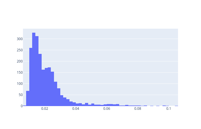
We now define the threshold.
threshold = np.mean(train_loss) + np.std(train_loss)
print("Threshold: ", threshold)
Threshold: 0.028107813
On the test dataset, we will use the threshold above to determine anormalies. We will do this as follows:
reconstructions_normal = autoencoder.predict(normal_test_data)
test_loss_normal = tf.keras.losses.mae(reconstructions_normal, normal_test_data)


reconstructions_abnormal = autoencoder.predict(abnormal_test_data)
test_loss_abnormal = tf.keras.losses.mae(reconstructions_abnormal, abnormal_test_data)

fig = go.Figure()
fig.add_trace(go.Histogram(x=test_loss_normal[None,:][0],name='Normal loss'))
fig.add_trace(go.Histogram(x=test_loss_abnormal[None,:][0],name='Abnormal loss',opacity=0.4))

# Overlay both histograms
fig.update_layout(barmode='overlay')
# Reduce opacity to see both histograms
fig.update_traces(opacity=0.75)


fig.add_shape(type="line",
    xref="x", yref="y",
    x0=threshold, y0=0, x1=threshold, y1=90,
    line=dict(
        color="red",
        width=3,
    ),
)
fig.show()
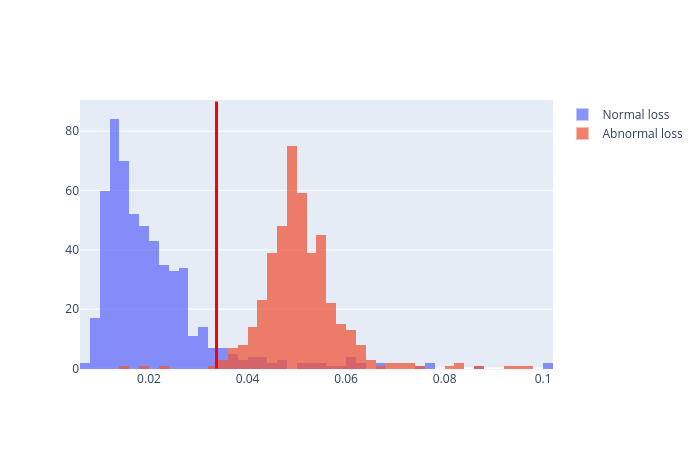
The red vertical line is at the threshold. Anything above the red vertical line is considered as an anormaly.
How accurate is our model
We will compute the accuracy, precision and recall of our model.
def predict(model, data, threshold):
  reconstructions = model(data)
  loss = tf.keras.losses.mae(reconstructions, data)
  return tf.math.less(loss, threshold)

def print_stats(predictions, labels):
  print("Accuracy = {}".format(accuracy_score(labels, predictions)))
  print("Precision = {}".format(precision_score(labels, predictions)))
  print("Recall = {}".format(recall_score(labels, predictions)))


preds = predict(autoencoder, test_data, threshold)
print_stats(preds, test_labels)
Accuracy = 0.939
Precision = 0.994059405940594
Recall = 0.8964285714285715
The complete notebook can be found here.
Final words
In this blog post, we have seen how autoencoders can be used to detect anomalies in our data. The ECG data is a nice example to illustrate the idea, however, with a typical real-world use case, there will be more shortcomings.